Regularization
Any technique to reduce generalization error but not training error.
Parameter norm penalties:
$\tilde J = J + \alpha\Omega$ where the $\alpha\Omega$ term describes the penalty.
We do not regularize biases, because they only affect the output. Regularizing weights can lead to underfitting. Weights are a relation between inputs and outputs, and thus require more datapoints to gather a relationship.
L2 regularization
$$ \Omega = \frac{1}{2}||w||^2 $$
Gradient:
$$ \nabla_w \tilde J = \nabla_w J + \alpha w\nabla_w w = \nabla_w J + \alpha w $$
Gradient step:
$$ w \leftarrow w - \epsilon (\alpha w + \nabla_w J) \ = w(1-\epsilon \alpha) - \epsilon\nabla_w J $$
- effectively “shrinks” weights before applying gradient step
$\tilde w = Q(\Lambda + \alpha I)^{-1} \Lambda Q^T w^*$ so $\alpha$ rescales the eigenvalues by $\lambda / (\lambda + \alpha)$. Small $\lambda$ are heavily penalized, large $\lambda$ aren’t.
Linear regression
cost = $||Xw-y||^2$ and after applying L2 regularization, this becomes $||Xw-y||^2 + \frac{1}{2}\alpha||w||^2$.
Solution becomes $w=(X^TX + \alpha I)^{-1} X^T y$, where $\frac{1}{m}X^TX$ is the covariance matrix.
Effectively adding $\alpha$ to each diagonal element (each variance increases); also useful for making the matrix non-singular.
L1 regularization
$$ \Omega = ||w||_1 = \sum_i |w_i| $$
$$ \nabla_w \tilde J = \nabla_w J + \text{asign}(w) \nabla_w \tilde J = H(w - w*) $$
- H = Hessian matrix
Assume H is diagonal (can be done using PCA). Using quadratic approximation,
$$\tilde J = J + \sum_i \frac{1}{2} H_{ii}(w_i-w_i^*) + \alpha|w_i|$$
The solution is
$$w_i = \text{sign}(w_i*)\max{|w_i^*| - \frac{a}{H_{ii}}, 0}$$
If $|w_i^*| < \frac{a}{H_{ii}}$, then $w_i = 0$, because $\tilde J$ is overwhelmed by the regularization; otherwise it moves towards 0.
L1 regularization can set weights to zero (sparse).
Can be used for feature selection (e.g. LASSO).
Explicit constraints vs. Penalties
Penalties can result in local minima with “dead” neurons, which have small weights in and out.
Constraints + descending on J and reprojecting is often more useful.
Dataset Augmentation
Increase generalization by transforming training data to get more samples. Examples include:
- translating, rotation, and scaling images
- adding noise
- dropout
Noise Robustness
Noise encourages the algorithm to find areas stable to perturbations - local minima surrounded by flatness.
Output Target Noise
You can also apply noise to the output.
Label smoothing: replace 0, 1 with $\epsilon/(k-1)$, $1-\epsilon$.
If using maximum likelihood, your algorithm may never converge and norm may go to infinity, so use a norm regularizer as well.
Early Stopping
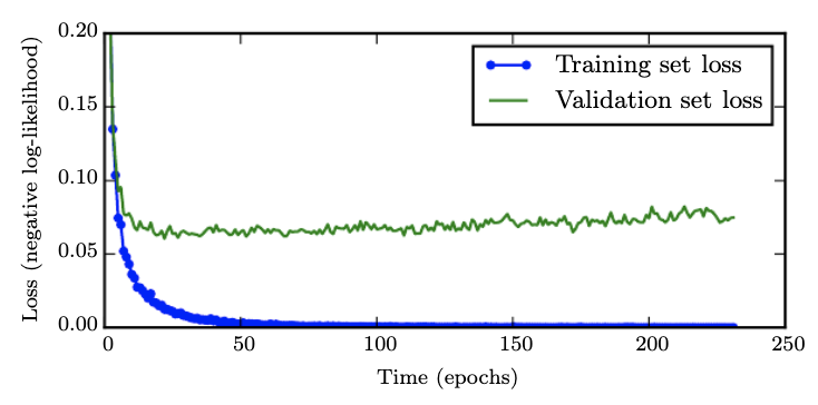
As epochs increase, validation error goes down and then up. We can stop training our model at the lowest validation set loss.

Parameters that correspond to significant curvature are “more important” and are learned faster than parameters that correspond to less curvature.
Parameter Sharing
Two different models can share parameters. This:
- captures relationship between them
- reduces memory
Sparse Representations
Make the data in x sparse by applying some function f: y = Ax, where x has many zeroes.
Bagging
- Also known as bootstrap averaging.
Reduces generalization error by combining several different models.
Train the separate models, then have the models vote on the output.
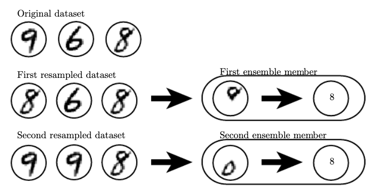
This is an example of model averaging, and techniques employing this strategy are known as ensemble methods.
Why is this effective? Different models won’t make the same errors (generally). Consider k models, each with an error e~i~ on each example such that $\mathbb{E}[e_i^2] = v$ and $\mathbb{E}[e_ie_j] = c$. Then, the expected error is
$$ \mathbb{E}[(\frac{1}{k}\sum e_i)^2] = \frac{1}{k^2}\mathbb{E}[\sum e_i^2 + \sum_{i \neq j}e_ie_j] \ = \frac{1}{k}v + \frac{k-1}{k}c $$
If $c = v$, then we get the error is v, so it is no worse. However, for $c \leq v$, the error decreases.
Implementation
Bagging involves constructing k different datasets, each of which is a sample with replacement from the original dataset.

Benchmarks usually omit bagging because every algorithm benefits from it. However, it is more memory/time intensive.
Dropout
Removes units from a neutral network randomly.
In practice, this is done by randomly generating a random binary mask at each training step.
- Usually, p = 0.8 for inputs and p=0.5 for hidden layers
- Form of parameter sharing
Similar to bagging - this method trains an exponential # of models without using much memory.
Another way to view droput:
- Hidden units must be able to perform well, regardless of adjacent units
- Similiar to sexual reproduction - genes are robust with respect to other genes
- Features must be good in many contexts
Weight Scaling Inference Rule
To predict a distribution $p$, it is necessary to normalize our prediction $\tilde p$. To approximate this, we can multiply weights out of a node i by multiplying the probability of including i.
Empirically, this works very well, but there is no strong theoretical reason why it works (however, this is exact for linear models).
Adversarial Training

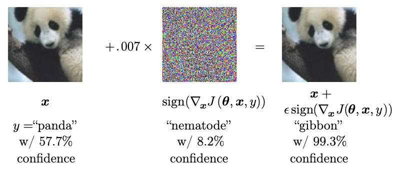
Given a model and a point x, search for a point x’ near x such that the output is very different at x'.
This forces nonlinearity, because linear functions can be very sensitive to small e: e||w|| can be large, especially if w is high-dimensional.